Today I would be talking about device tree:
Device Tree is a data structure by which bootloaders pass
hardware layout to Linux in a device-independent manner, simplifying hardware
probing.
Mailing list for device tree is mailing list at:
https://lists.ozlabs.org/listinfo/devicetree-discuss
Introduction:
During development of Linux/ppc64 kernel it was decided to enforce some strict rules regarding the kernel entry point and bootloader <-> kernel interface,in order to avoid degeneration that become the ppc32 kernel entry point and the way a new platform should be added to the kernel.
-device-tree whose format is defined after Open Firmware specification.
-To make easy the kernel does not required the device tree to represent every device.Only some nodes and properties to be present.
-For example the kernel does not require to create a node for every PCI device.It will create node for PCI Host bridges which provides information for interrupt routing information and memory I/O ranges among others.
-It is recomended to specify nodes for chip devices and other devices and other Bus that does not fit into existing OF specification.
-This creates the flexibility in the way the kernel can then probe those and match drivers to device,without having hard code all sorts of tables.
-Also makes flexible for board vendors to do minor hardware upgrades without significanltly impacting the kernel code or clustering it with special cases.
1)Entry point for arch/arm:
There is single entry point to the kernel,at the start of the kernel image.That entry point has two calling convention.
a)ATAGS interface:
Minimal information is passed from firmware ->kernel with a tagged list of predefined parameters.
r0=0
r1=Machine type number
r2=Physical address of tagged list in system RAM
b)entry of device tree.Firmware loads the physical address of the device tree block(dtb) into r2.R1 is not used but it is considers as good practice to use valid machine number.
r0=0
r1=valid machine type number. When using device tree a single machine type number will often be assigned to represent a class or family of SOCs.
r2=physical pointer to the device tree in RAM.It can be located on anywhere in system RAM, but it should be aligned on 64-bit boundary.
-Kernel will differentiate between ATAGS and device tree booting by reading the memory pointed to by r2 and looking for either the device tree Block magic value(0xd00dfeed) or the ATAG_CORE value at offset 0x4 from r2(0x54410001)
The kernel is passed the physical address pointing to an area of memory
that is roughly described in include/linux/of_fdt.h by the structure
boot_param_header:
struct boot_param_header {
u32 magic; /* magic word OF_DT_HEADER */
u32 totalsize; /* total size of DT block */
u32 off_dt_struct; /* offset to structure */
u32 off_dt_strings; /* offset to strings */
u32 off_mem_rsvmap; /* offset to memory reserve map
*/
u32 version; /* format version */
u32 last_comp_version; /* last compatible version */
/* version 2 fields below */
u32 boot_cpuid_phys; /* Which physical CPU id we're
booting on */
/* version 3 fields below */
u32 size_dt_strings; /* size of the strings block */
/* version 17 fields below */
u32 size_dt_struct; /* size of the DT structure block */
};
/* Definitions used by the flattened device tree */
#define OF_DT_HEADER 0xd00dfeed /* 4: version,4: total size */
#define OF_DT_BEGIN_NODE 0x1 /* Start node: full name*/
#define OF_DT_END_NODE 0x2 /* End node */
#define OF_DT_PROP 0x3 /* Property: name off,size, content */
#define OF_DT_END 0x9
- magic
This is a magic value that "marks" the beginning of the
device-tree block header. It contains the value 0xd00dfeed and is
defined by the constant OF_DT_HEADER
- totalsize
This is the total size of the DT block including the header. The
"DT" block should enclose all data structures defined in this
chapter (who are pointed to by offsets in this header). That is,
the device-tree structure, strings, and the memory reserve map.
-off_dt_struct
This is an offset from the beginning of the header to the start
of the "structure" part the device tree.
- off_dt_strings
This is an offset from the beginning of the header to the start
of the "strings" part of the device-tree
- off_mem_rsvmap
This is an offset from the beginning of the header to the start
of the reserved memory map. This map is a list of pairs of 64-
bit integers. Each pair is a physical address and a size. The
list is terminated by an entry of size 0. This map provides the
kernel with a list of physical memory areas that are "reserved"
and thus not to be used for memory allocations, especially during
early initialization. The kernel needs to allocate memory during
boot for things like un-flattening the device-tree, allocating an
MMU hash table, etc... Those allocations must be done in such a
way to avoid overriding critical things like, on Open Firmware
capable machines, the RTAS instance, or on some pSeries, the TCE
tables used for the iommu. Typically, the reserve map should
contain _at least_ this DT block itself (header,total_size). If
you are passing an initrd to the kernel, you should reserve it as
well. You do not need to reserve the kernel image itself. The map
should be 64-bit aligned.
- version
This is the version of this structure. Version 1 stops
here. Version 2 adds an additional field boot_cpuid_phys.
Version 3 adds the size of the strings block, allowing the kernel
to reallocate it easily at boot and free up the unused flattened
structure after expansion. Version 16 introduces a new more
"compact" format for the tree itself that is however not backward
compatible. Version 17 adds an additional field, size_dt_struct,
allowing it to be reallocated or moved more easily (this is
particularly useful for bootloaders which need to make
adjustments to a device tree based on probed information). You
should always generate a structure of the highest version defined
at the time of your implementation. Currently that is version 17,
unless you explicitly aim at being backward compatible.
- last_comp_version
Last compatible version. This indicates down to what version of
the DT block you are backward compatible. For example, version 2
is backward compatible with version 1 (that is, a kernel build
for version 1 will be able to boot with a version 2 format). You
should put a 1 in this field if you generate a device tree of
version 1 to 3, or 16 if you generate a tree of version 16 or 17
using the new unit name format.
- boot_cpuid_phys
This field only exist on version 2 headers. It indicate which
physical CPU ID is calling the kernel entry point. This is used,
among others, by kexec. If you are on an SMP system, this value
should match the content of the "reg" property of the CPU node in
the device-tree corresponding to the CPU calling the kernel entry
point (see further chapters for more information on the required
device-tree contents)
- size_dt_strings
This field only exists on version 3 and later headers. It
gives the size of the "strings" section of the device tree (which
starts at the offset given by off_dt_strings).
- size_dt_struct
This field only exists on version 17 and later headers. It gives
the size of the "structure" section of the device tree (which
starts at the offset given by off_dt_struct).
------------------------------
base -> | struct boot_param_header |
------------------------------
| (alignment gap) (*) |
------------------------------
| memory reserve map |
------------------------------
| (alignment gap) |
------------------------------
| |
| device-tree structure |
| |
------------------------------
| (alignment gap) |
------------------------------
| |
| device-tree strings |
| |
-----> ------------------------------
|
|
--- (base + totalsize)
(*) The alignment gaps are not necessarily present; their presence
and size are dependent on the various alignment requirements of
the individual data blocks.
2:Device Tree generalites
This device-tree itself is separate in two different blocks:
1)structure block
2)string block
Both are alinged to 4 byte boundary
What is device-tree?
-Its basically a tree of nodes, each node having two or more named properties.A property can have value or not.
-It is a tree so each node has one parent while otherwise they dont have node.
-Node has two names.
Actual node name is generally contained in the property "name" in the node property list(whose value is zero terminated and it is mandatory in for version 1 to 3)
-from version 16 its optional.(it generates from unit name defined below)
-Another name is "unit name" that is used to differentiate nodes with same name at the same level.
-It is usually made of "nodes name" then @ then "unit address",which defination is specific to bus type the node sits on.
-Unit name does not exist as property per-se but it is included in device tree structure.That is typically used to represent path in device-tree.
-Kernel generic code does not uses unit address so the only real requirment here for unit address is to ensure uniqueness of the node unit name at the given level of the tree.
-The node with no notion of address and no possible sibling of the same name may omit the unit address in the context of the specification or use "@0" defualt unit address.
- The unit name is used to define a node "full path", which is the concatenation of all parent node unit names separated with "/".
Root node
-The root node doesn't have a defined name.It also has no unit address.The root node unit name is thus an empty string. The full path to the root node is "/".
-Every node which actually represents an actual device is also required to have a "compatible" property indicating the specific hardware and an optional list of devices it is fully backwards compatible with.
-every node that can be referenced from a property in another node is required to have either a "phandle" or a "linux,phandle"
-Here is the example of the device tree
/ o device-tree
|- name = "device-tree"
|- model = "MyBoardName"
|- compatible = "MyBoardFamilyName"
|- #address-cells = <2>
|- #size-cells = <2>
|- linux,phandle = <0>
|
o cpus
| | - name = "cpus"
| | - linux,phandle = <1>
| | - #address-cells = <1>
| | - #size-cells = <0>
| |
| o PowerPC,970@0
| |- name = "PowerPC,970"
| |- device_type = "cpu"
| |- reg = <0>
| |- clock-frequency = <0x5f5e1000>
| |- 64-bit
| |- linux,phandle = <2>
|
o memory@0
| |- name = "memory"
| |- device_type = "memory"
| |- reg = <0x00000000 0x00000000 0x00000000 0x20000000>
| |- linux,phandle = <3>
|
o chosen
|- name = "chosen"
|- bootargs = "root=/dev/sda2"
|- linux,phandle = <4>
o -represents the device tree. Followed by the node unit name
property are followed by the name and then followed by the content.
"content"-represents as ACSII type
<>-represents a 32 bit value in decimal or hexadecimal.
3:Structure Block
The structure of the device tree is linearized tree structure.
"OF_DT_BEGIN_NODE" token starts a new node
"OF_DT_END_NODE" ends that node definition
Child nodes are simply defined before "OF_DT_END_NODE"
Here's the basic structure of a single node:
* token OF_DT_BEGIN_NODE (that is 0x00000001)
* for version 1 to 3, this is the node full path as a zero
terminated string, starting with "/". For version 16 and later,
this is the node unit name only (or an empty string for the
root node)
* [align gap to next 4 bytes boundary]
* for each property:
* token OF_DT_PROP (that is 0x00000003)
* 32-bit value of property value size in bytes (or 0 if no
value)
* 32-bit value of offset in string block of property name
* property value data if any
* [align gap to next 4 bytes boundary]
* [child nodes if any]
* token OF_DT_END_NODE (that is 0x00000002)
So the node content can be summarized as a start token,full path, a list of properties, a list of child nodes, and a end token.Every child node is the full structure itself as defined above.
4:Device tree "string" block
-In order to save space,property names,which are generally redundant are stored seperatly in the "strings" block.
-This block is simply whole bunch of zero terminated strings for all properties name concatenated together.
-The device-tree property definition in the stucture block will contain offset values from beginning of the string block.
--------------------------------------------------------------------------------------------------------------------
Required content of the device tree:
WARNING:All 'linux' properties defined in this document apply to device tree.If your platform uses a real implementation of open firmware or an implementation compatible with the open firmware client interface,those properties will be created by the trampoline code in the kernel prom_init() file For example, that's where you'll have to add code to detect your board model and set the platform number. However, when using the flattened device-tree entry point, there is no prom_init() pass, and thus you have to provide those properties yourself.
1)Note about cells and address representation:
The general rule is documentaed in open firmware documentation.
-If you choose a bus with the device tree and there exit OP bus binding,then you should follow specification.However kernel does not need to describe every device in device tree.
Format of address is defined my the parent bus type,based on #address-cell and #size-cell. These address are not inherited from parent so note that so every node with children must specify them.
What is cell?
Those 2 properties define 'cells' for representing an address and a size. A "cell" is a 32-bit number. For example, if both contain 2 like the example tree given above, then an address and a size are both composed of 2 cells, and each is a 64-bit number (cells are concatenated and expected to be in big endian format). Another example
is the way Apple firmware defines them, with 2 cells for an address and one cell for a size. Most 32-bit implementations should define #address-cells and #size-cells to 1, which represents a 32-bit value. Some 32-bit processors allow for physical addresses greater than 32 bits; these processors should define #address-cells as 2.
2)Note about "compatiblle" property
These properties are optional, but recommended in device and the root node. The format of "compatible" property is a list of concatenated zero terminated strings. They allow a device to express its compatibility with family of similar device.n some cases,allowing a single driver to match against several devices regardless
of their actual names.
3)Note on "name" property
-While earlier users of Open Firmware like OldWorld macintoshes tended
to use the actual device name for the "name" property, it's nowadays
considered a good practice to use a name that is closer to the device
class (often equal to device_type). For example, nowadays, Ethernet
controllers are named "ethernet", an additional "model" property
defining precisely the chip type/model, and "compatible" property
defining the family in case a single driver can driver more than one
of these chips. However, the kernel doesn't generally put any
restriction on the "name" property; it is simply considered good
practice to follow the standard and its evolutions as closely as
possible.
-Note also that the new format version 16 makes the "name" property
optional. If it's absent for a node, then the node's unit name is then
used to reconstruct the name. That is, the part of the unit name
before the "@" sign is used (or the entire unit name if no "@" sign
is present).
4) Note about node and property names and character set
-------------------------------------------------------
The root node requires some properties to be present:
- model : this is your board name/model
- #address-cells : address representation for "root" devices
- #size-cells: the size representation for "root" devices
- compatible : the board "family" generally finds its way here,
for example, if you have 2 board models with a similar layout,
that typically get driven by the same platform code in the
kernel, you would specify the exact board model in the
compatible property followed by an entry that represents the SoC
model.
The root node is also generally where you add additional properties
specific to your board like the serial number if any, that sort of
thing. It is recommended that if you add any "custom" property whose
name may clash with standard defined ones, you prefix them with your
vendor name and a comma.
b) The /cpus node
This node is the parent of all individual CPU nodes. It doesn't
have any specific requirements, though it's generally good practice
to have at least:
#address-cells = <00000001>
#size-cells = <00000000>
This defines that the "address" for a CPU is a single cell, and has
no meaningful size. This is not necessary but the kernel will assume
that format when reading the "reg" properties of a CPU node, see
below
c) The /cpus/* nodes
-So under /cpus, you are supposed to create a node for every CPU on
the machine.
-So under /cpus, you are supposed to create a node for every CPU on
the machine
-So under /cpus, you are supposed to create a node for every CPU on
the machine
-the Generic Names convention suggests that it would be
better to simply use 'cpu' for each cpu node and use the compatible
property to identify the specific cpu core.
Required properties:
- device_type : has to be "cpu"
- reg : This is the physical CPU number, it's a single 32-bit cell
and is also used as-is as the unit number for constructing the
unit name in the full path. For example, with 2 CPUs, you would
have the full path:
/cpus/PowerPC,970FX@0
/cpus/PowerPC,970FX@1
(unit addresses do not require leading zeroes)
- d-cache-block-size : one cell, L1 data cache block size in bytes (*)
- i-cache-block-size : one cell, L1 instruction cache block size in
bytes
- d-cache-size : one cell, size of L1 data cache in bytes
- i-cache-size : one cell, size of L1 instruction cache in bytes
(*) The cache "block" size is the size on which the cache management instructions operate. Historically, this document used the cache "line" size here which is incorrect. The kernel will prefer the cache block size and will fallback to cache line size for backward compatibility.
Recommended properties:
- timebase-frequency : a cell indicating the frequency of the
timebase in Hz. This is not directly used by the generic code,
but you are welcome to copy/paste the pSeries code for setting
the kernel timebase/decrementer calibration based on this
value.
- clock-frequency : a cell indicating the CPU core clock frequency
in Hz. A new property will be defined for 64-bit values, but if
your frequency is < 4Ghz, one cell is enough. Here as well as
for the above, the common code doesn't use that property, but
you are welcome to re-use the pSeries or Maple one. A future
kernel version might provide a common function for this.
- d-cache-line-size : one cell, L1 data cache line size in bytes
if different from the block size
- i-cache-line-size : one cell, L1 instruction cache line size in
bytes if different from the block size
 Remove these ads by

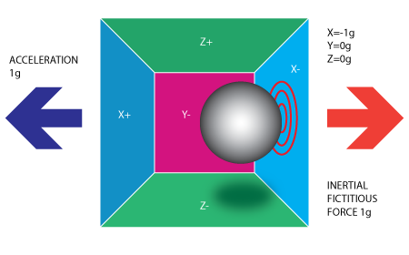
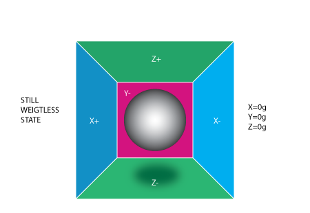 If we take this box in a place with no gravitation fields or for that
matter with no other fields that might affect the ball's position - the
ball will simply float in the middle of the box. You can imagine the
box is in outer-space far-far away from any cosmic bodies, or if such a
place is hard to find imagine at least a space craft orbiting around the
planet where everything is in weightless state . From the picture above
you can see that we assign to each axis a pair of walls (we removed the
wall Y+ so we can look inside the box). Imagine that each wall is
pressure sensitive. If we move suddenly the box to the left (we
accelerate it with acceleration 1g = 9.8m/s^2), the ball will hit the
wall X-. We then measure the pressure force that the ball applies to the
wall and output a value of -1g on the X axis.
If we take this box in a place with no gravitation fields or for that
matter with no other fields that might affect the ball's position - the
ball will simply float in the middle of the box. You can imagine the
box is in outer-space far-far away from any cosmic bodies, or if such a
place is hard to find imagine at least a space craft orbiting around the
planet where everything is in weightless state . From the picture above
you can see that we assign to each axis a pair of walls (we removed the
wall Y+ so we can look inside the box). Imagine that each wall is
pressure sensitive. If we move suddenly the box to the left (we
accelerate it with acceleration 1g = 9.8m/s^2), the ball will hit the
wall X-. We then measure the pressure force that the ball applies to the
wall and output a value of -1g on the X axis.